Entropy as Disorganization and Mixture
Info Energy employed to maintain Gains
In the article Integration: Living Algorithm Dynamics we discussed efficiency in the Living Algorithm System. We mentioned that info efficiency is quite low as compared with physical efficiency.
Why?
Efficiency is the ratio of Power to Energy. The greater the Power relative to the total Energy expenditure, the greater the Efficiency, and vice versa. This relationship holds true for the dynamics of both information and matter.
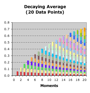
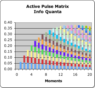
The Living Average Grid at left is a visualization of the Info Energy Quanta of a data stream consisting of 20 1s (the beginning of the Active Pulse). Summing the info energy columns reveals how much info energy has been expended at any Moment in the data stream. The Directional Grid at right is a visualization of the Info Force Quanta of the same data stream. When Attention is sustained over time, the force quanta accumulate to become columns of info work. Summing these info work columns over time yields the info power of the System at any Moment. Comparing these Grids, one energy-based and the other power-based, will reveal the relationship between Energy and Power in the Living Algorithm System (at least when the data stream consists of 20 1s).
100% Efficiency (Energy Consumed/Power) impossible due to Entropy
Dividing Power by the Total Energy in the System determines Efficiency. Hence a highly efficient system is one in which power is close in size to total energy. Carnot and others showed that even for physical systems that 100% efficiency is an impossible ideal due to a mysterious construct known as entropy.
Entropy: the innate decrease in System's organization over time
Under one perspective, entropy is the innate decrease in the organization of a system that occurs naturally over time. The energy is still in the system. It is just not as organized. Energy has not been lost. This would violate the well-established law of energy conservation. It's just less organized. This innate loss of organization with time is why physical systems can never be 100% efficient - no perpetual motion machines.
Innate feature of Disorganization is Mixture
An innate feature of disorganization is mixture. Organization implies differentiation. As an example: the Dewey Decimal System is a highly organized system that differentiates books into ever finer categories for easy reference at libraries. At home our books are generally more mixed up. This mixture reveals a higher level of entropy. If some kind of disaster, for instance an earthquake, toppled our bookshelves, the resulting disorganization would lower the organization of our system even further. Although the books would remain the same, the entropy of the system increases. Another example: Our walls frequently separate the cooler outside temperature (the sedate gas molecules) from the warmer inside temperature (the excited gas molecules). This state is more organized and has less entropy than when internal and external temperatures are mixed. When the door or windows are left open the entropy rises because the excited gas molecules mix their energy with the sedate gas molecules.
Info Entropy: a type of Mixture
This same mixture is what diminishes the ratio of Info Power to Info Energy. Accordingly, we will refer to this as info entropy, as applied to the data stream dynamics of the Living Algorithm System. Let's see how the Living Algorithm process disorganizes the quanta of Info Energy.
Graphic Visualization: Power Quanta reduction relative to Energy Quanta
Graph: Energy Quanta vs. Force Quanta over 11 moments
As visualization frequently leads understanding, let's view our quanta grids in more detail, before examining the algebra behind the entropic process.
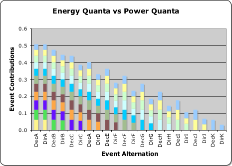
The above graph offers a comparison of the amount of energy quanta versus the amount of force (power) quanta that the Living Algorithm System consumes over 11 moments. The columns break the consumption into individual Events. The 1st column represents Event A's energy contribution (DecA) to the System during the first 11 moments in the data stream. The 2nd column represents Event A's power contribution (DirA) to the System during the first 11 moments in the data stream. The 3rd column represents Event B's energy contribution (DecB) and the 4th column represents Event B's power contribution (DirB) to the System during the first 11 moments. This alternation of energy and power quanta from successive Events continues through the 11th Event (Event K).
Colored Rectangles = Consumed Energy and Power Quanta
The colored rectangles represent the info or force quanta that are consumed at each moment along the way. For instance, the info quanta (the colored rectangles) along the bottom of the graph represent the initial Impact of each Event, whether energy or force quanta. The 2nd row of info quanta represents the 1st Influence of each Event (the scaled Impact). The 3rd row of info quanta represents the 2nd Influence of each Event (the scaled 1st Influence). The pattern continues. Notice that this graph is organized by Events, not by Moments.
Power Impact and subsequent Influences become smaller and smaller
There are a few striking features to the graph. 1) As we move to the right in the graph, the initial Impact of the power quantum becomes smaller and smaller relative to the initial Impact of the energy quantum, which remains the same throughout. 2) This reduction in size is reflected in the subsequent Power Influences that are piled on top of the Impact in each column. 3) As we move to the right, the total contribution of the Power Events shrinks in comparison to the Energy Events.
With each Iteration more info energy for maintenance & less for change = Less Power
The successive shrinkage of the Power Impacts with each iteration means that each new Event employs less of its energy to change the system and more of its energy to maintain the State of the System. This shift is because part of the info energy must be continually employed to reduce the impact of the Decay Factor. Employing an increasing amount of energy on maintenance means that the incoming info energy does less and less work. A reduction in the info energy's work translates into less power. When power is reduced in relation to energy, the efficiency of the System falls. Accordingly, this peculiar mathematical process is the root of the loss in efficiency in our System. Now that we have visualized the process, let us examine the algebra behind this intriguing process.
Algebra: Power's Impact Quanta reduction relative to Energy's Impact Quanta
Living Average Events at 3rd Moment
Directional Events at 3rd Moment
It is time to talk about info entropy from the uniquely specific perspective of mathematics.
The 3rd Moment from an Event Perspective
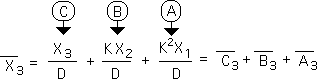
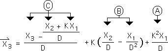
Let's look at a specific example of info entropy to better understand the process. We are going to examine the differences between the Living Average (X3 bar – the 1st derivative) and the Directional (X3 arrow – the 2nd derivative) at the 3rd moment. Equations 3.15 & 3.16 view these data stream derivatives from the Event perspective.
Living Average Events Pure; Directional Events polluted by prior Data
As mentioned in an earlier article, the Living Average Events are functions of the data that spawned them - with no other polluting factors. In contrast, the Directional Events are functions of the data that spawned them combined with all the data from the preceding Events. In other words the Directional Events are not pure, but are instead a mixture of new and old data. As we shall see, this mixture is the basis of info entropy.
Event A is identical for Living Average and Directional, as no prior data
5.1 Let's be more specific. Event A is identical for the Decay Average and the Directional at the 3rd moment. This makes sense. As the 1st Event, there is no prior data to disorganize to System. Further, the Living Average's Event A is always identical to the Directional' Event A at every moment, as Event Influences (the info quanta) go through the identical process, scaling by K.

Directional's Event B is Living Average's Event B scaled once.
5.2 The 1st element in the Directional's Event B is identical to the Living Average's Event B. However, the 2nd element is a subtraction (shown at right). This reduction is due to the 'polluting' influence of the prior data byte. If the data bytes are identical (as in the Active Pulse of 1s), the Directional B is simply a scaled (multiplied by K, the Scaling Factor) version of Living Average B at the 3rd moment. This reasoning applies to all subsequent Influences in Event B as well. Each Directional B is scaled once in relationship to Living Average A. This scaling (reduction) is due to the 'polluting' influence of prior data - the entropic mixing of the old with the new.

Note there is no reduction in the info energy. It is just used less efficiently. This reduction in power is inherent to the algebra of the Living Algorithm's digestive process.
Directional C = Living Average C scaled twice
5.3 Let's continue our analysis with Event C. The same parallels hold when we compare Living Average C and Directional C. The 1st element in both Events is identical. However, Directional C is diminished by the 'polluting' influence of 2 prior data points. This entropic mixture reduces the size of Event C's power quantum, hence the efficiency of the System. When the data bytes are equal (as in the Active Pulse), the power quanta in Directional C are scaled twice (multiplied by K twice, K2) in comparison to the energy quanta in Living Average C. The Directional's power quanta are further reduced in comparison with the Living Average's energy quanta. This relationship holds for every subsequent Influence in Event C.

General Equation for the relationship between parallel Power Quanta and Energy Quanta
5.4 With each new Event, the power quanta are scaled yet another time in comparison with the energy quanta. For instance, in Event D the power quanta are scaled 3 times (K3) and in Event E the power quanta are scaled 4 times in comparison to the energy quanta. When a power quantum and an energy quantum are associated with the same Moment and the same Event, they are said to be parallel quantum. The general equation of the relationship between parallel power quanta and energy quanta when the Data is identical is shown below. This relationship applies to the Active Pulse of 1s.

Successive Scaling of Power Quanta versus Energy Quanta is the Root of Info Entropy
It is evident that the System loses more power with each iteration of the Living Algorithm process. Hence, the efficiency is reduced accordingly. This successive scaling of power quanta versus energy quanta is the root of info entropy. It is an innate feature of the Living Algorithm's digestion process.
No Info Energy Lost, just employed on maintenance rather than change
Reiterating for memory: no info energy is lost. The info energy quanta from the Living Average Grid are eventually consumed completely. The info energy is used to change and maintain the system. There is no power in maintenance. The more energy that is employed to maintain the state of the System, the less energy that is employed to change the System. The less energy is employed in change, the less power the System has. A reduction in power results in a reduction in efficiency. Although the efficiency is successively reduced, there is still power in an organized data stream. In contrast, random data streams have no power and no efficiency.
Generalization of Active Pulse
Triple Active Pulse from Core Concept article
In general, we have characterized the Active Pulse as the result when the Living Algorithm digests a series of uninterrupted 1s. The preceding algebraic analysis suggests that the Active Pulse is the result when the Living Algorithm digests any series of uninterrupted numbers. In other words, the Active Pulse is the result when the Living Algorithm digests an uninterrupted series of 4, 5, or any other number N. We first exhibited this phenomenon in our Core Concept article. When the Living Algorithm digested a series of 1s followed by a series of 2s followed by a series of 3s, the result was 3 Active Pulses – which we deemed the Triple Active Pulse. However, this example was merely a demonstration.
Striking algebraic simplifications when data stream members are equal
In the preceding articles, we examined what happened algebraically to energy and power quanta in the Living Algorithm System when the data stream is limited to a single common number. Simply speaking, all the numbers in the data stream are the same. With this simple restriction, we were able to come up with a general equation that computed the value of every power quantum. Remember the Active Pulse is a visualization of power quantum. In the current article we examined the relationship between energy quanta and power quanta when the data stream consists of equal members. Again we came up with a striking algebraic simplification for this relationship. In other words, we are not required to restrict our data stream to 1s to achieve this ultimate simplification. We only need restrict the data stream to a single number, any number.
Active Pulse: when the Living Algorithm digests a single number, not just ones
The combination of graphic visualization and algebraic simplification leads to the inescapable conclusion that the Active Pulse is the result when the Living Algorithm digests any uninterrupted series of numbers, not just 1s. The relationships between power and energy quanta are the same, no matter which number is employed. In other words the characteristic behavior of the Active Pulse remains the same no matter which number is digested. However, it must be the same number.
The state of N
In a prior article as a verbal simplification, we referred to an uninterrupted series of 1s as the state of 1, an uninterrupted series of 2s as the state of 2 and so on. In general when an uninterrupted series of any number N is sufficient to generate the Active Pulse, we will refer to this as the state of N.
Link
Now that we have examined Info Power and Efficiency as it applies to a data stream where the elements are equal, we can now investigate the impact of 'interruptions'. To find out the mathematics behind this intriguing phenomenon, read the next article in the series – Interruptions to the Active Pulse.